drawdf demonstration
drawdf is not yet available in the standard Maxima distribution,
but can be downloaded from http://www.netris.org/~mhw/maxima/drawdf.mac
| (%i1) | load(drawdf); |

| (%i2) | wxplot_size: [600,400]; |
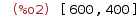
For convenience, drawdf and wxdrawdf accept most of the parameters
supported by plotdf.
| (%i3) | wxdrawdf(2*cos(t)-1+y, [t,-5,10], [y,-4,9], [trajectory_at,0,0])$ |
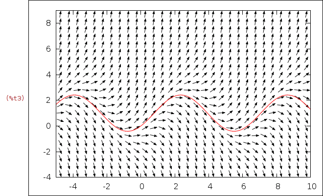
field_degree=2 causes the field to be composed of quadratic splines,
based on the first and second derivatives at each grid point.
soln_at() and solns_at() draw solution curves passing through the
specified points, using a slightly enhanced 4th-order Runge Kutta
numerical integrator.
| (%i4) |
wxdrawdf(2*cos(t)-1+y, [t,-5,10], [y,-4,9], field_degree=2, solns_at([0,0.1],[0,-0.1]), color=blue, soln_at(0,0))$ |
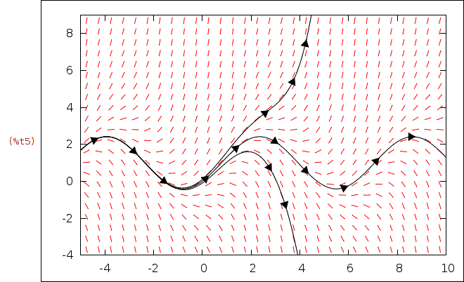
soln_arrows=true adds arrows to the solution curves, and (by default)
removes them from the direction field. It also changes the default
colors to emphasize the solution curves.
| (%i5) |
wxdrawdf(2*cos(t)-1+y, [t,-5,10], [y,-4,9], soln_arrows=true, solns_at([0,0.1],[0,-0.1],[0,0]))$ |
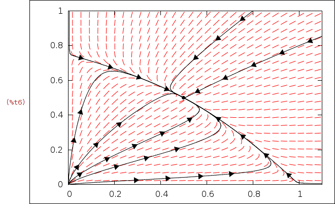
duration=40 specifies the time duration of numerical integration (default 10).
Integration will also stop automatically if the solution moves too far away
from the plotted region, or if the derivative becomes complex or infinite.
Here we also specify field_degree=2 to plot quadratic splines.
The equations below model a predator-prey system.
| (%i6) |
wxdrawdf([x*(1-x-y), y*(3/4-y-x/2)], [x,0,1.1], [y,0,1], field_degree=2, duration=40, soln_arrows=true, point_at(1/2,1/2), solns_at([0.1,0.2], [0.2,0.1], [1,0.8], [0.8,1], [0.1,0.1], [0.6,0.05], [0.05,0.4], [1,0.01], [0.01,0.75])) $ |
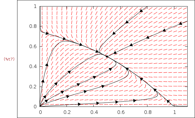
field_degree='solns causes the field to be composed of many small solution
curves computed by 4th-order Runge Kutta, with better results in this case.
| (%i7) |
wxdrawdf([x*(1-x-y), y*(3/4-y-x/2)], [x,0,1.1], [y,0,1], field_degree='solns, duration=40, soln_arrows=true, point_at(1/2,1/2), solns_at([0.1,0.2], [0.2,0.1], [1,0.8], [0.8,1], [0.1,0.1], [0.6,0.05], [0.05,0.4], [1,0.01], [0.01,0.75])) $ |
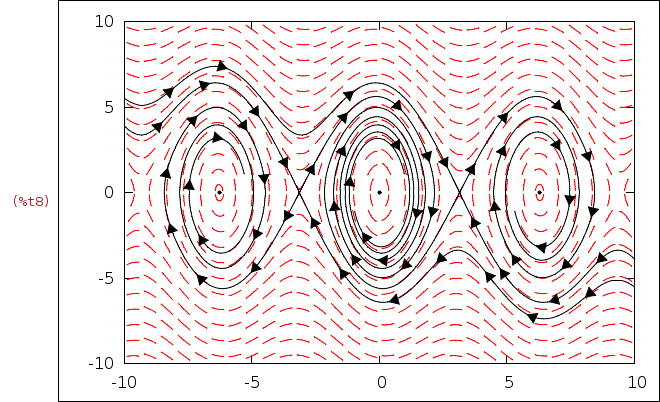
saddles_at() attempts to automatically linearize the equation at
each saddle, and to plot a numerical solution corresponding to each
eigenvector, including the separatrices. tstep=0.05 specifies the
maximum time step for the numerical integrator (the default is 0.1).
Note that smaller time steps will sometimes be used in order to keep
the x and y steps small. The equations below model a damped pendulum.
| (%i8) |
wxdrawdf([y,-9*sin(x)-y/5], tstep=0.05, soln_arrows=true, point_size=0.5, points_at([0,0], [2*%pi,0], [-2*%pi,0]), field_degree='solns, saddles_at([%pi,0], [-%pi,0]))$ |
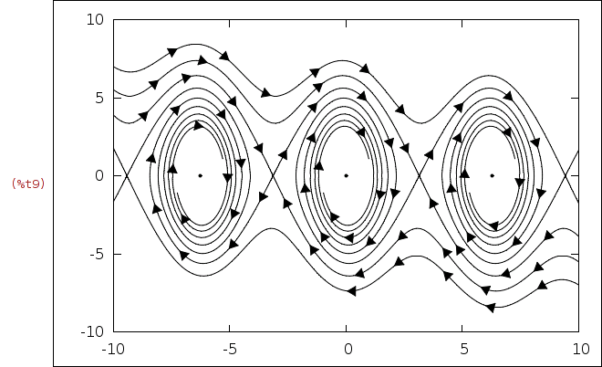
show_field=false suppresses the field entirely.
| (%i9) |
wxdrawdf([y,-9*sin(x)-y/5], tstep=0.05, show_field=false, soln_arrows=true, point_size=0.5, points_at([0,0], [2*%pi,0], [-2*%pi,0]), saddles_at([3*%pi,0], [-3*%pi,0], [%pi,0], [-%pi,0]))$ |
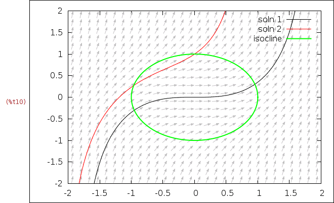
drawdf passes all unrecognized parameters to draw2d, allowing you
to combine the full power of the draw package with drawdf.
| (%i10) |
wxdrawdf(x^2+y^2, [x,-2,2], [y,-2,2], field_color=gray, key="soln 1", color=black, soln_at(0,0), key="soln 2", color=red, soln_at(0,1), key="isocline", color=green, line_width=2, nticks=100, parametric(cos(t),sin(t),t,0,2*%pi))$ |